Having examined the end systems and end-end transport service model of the Internet in Section 1.3, let us now delve more deeply into the "inside" of the network. In this section we study the network core--the mesh of routers that interconnect the Internet's end systems. Figure 1.4 highlights the network core in the thick, shaded lines.

Figure 1.4: The network core

1.4.1: Circuit Switching, Packet Switching, and Message Switching

There are two fundamental approaches towards building a network core: circuit switching and packet switching. In circuit-switched networks, the resources needed along a path (buffers, link bandwidth) to provide for communication between the end systems are reserved for the duration of the session. In packet-switched networks, these resources are not reserved; a session's messages use the resource on demand, and as a consequence, may have to wait (that is, queue) for access to a communication link. As a simple analogy, consider two restaurants--one that requires reservations and another that neither requires reservations nor accepts them. For the restaurant that requires reservations, we have to go through the hassle of first calling before we leave home. But when we arrive at the restaurant we can, in principle, immediately communicate with the waiter and order our meal. For the restaurant that does not require reservations, we don't need to bother to reserve a table. But when we arrive at the restaurant, we may have to wait for a table before we can communicate with the waiter.

The ubiquitous telephone networks are examples of circuit-switched networks. Consider what happens when one person wants to send information (voice or facsimile) to another over a telephone network. Before the sender can send the information, the network must first establish a connection between the sender and the receiver. In contrast with the TCP connection that we discussed in the previous section, this is a bona fide connection for which the switches on the path between the sender and receiver maintain connection state for that connection. In the jargon of telephony, this connection is called a circuit. When the network establishes the circuit, it also reserves a constant transmission rate in the network's links for the duration of the connection. This reservation allows the sender to transfer the data to the receiver at the guaranteed constant rate.

Today's Internet is a quintessential packet-switched network. Consider what happens when one host wants to send a packet to another host over a packet-switched network. As with circuit switching, the packet is transmitted over a series of communication links. But with packet switching, the packet is sent into the network without reserving any bandwidth whatsoever. If one of the links is congested because other packets need to be transmitted over the link at the same time, then our packet will have to wait in a buffer at the sending side of the transmission line, and suffer a delay. The Internet makes its best effort to deliver the data in a timely manner, but it does not make any guarantees.

Not all telecommunication networks can be neatly classified as pure circuit-switched networks or pure packet-switched networks. For example, for networks based on the ATM technology, a connection can make a reservation and yet its messages may still wait for congested resources! Nevertheless, this fundamental classification into packet- and circuit-switched networks is an excellent starting point in understanding telecommunication network technology.

Circuit Switching

This book is about computer networks, the Internet, and packet switching, not about telephone networks and circuit switching. Nevertheless, it is important to understand why the Internet and other computer networks use packet switching rather than the more traditional circuit-switching technology used in the telephone networks. For this reason, we now give a brief overview of circuit switching.

Figure 1.5 illustrates a circuit-switched network. In this network, the three circuit switches are interconnected by two links; each of these links has n circuits, so that each link can support n simultaneous connections. The end systems (for example, PCs and workstations) are each directly connected to one of the switches. (Ordinary telephones are also connected to the switches, but they are not shown in the diagram.) Notice that some of the hosts have analog access to the switches, whereas others have direct digital access. For analog access, a modem is required. When two hosts desire to communicate, the network establishes a dedicated end-to-end circuit between two hosts. (Conference calls between more than two devices are, of course, also possible. But to keep things simple, let's suppose for now that there are only two hosts for each connection.) Thus, in order for host A to send messages to host B, the network must first reserve one circuit on each of two links. Each link has n circuits; each end-to-end circuit over a link gets the fraction 1/n of the link's bandwidth for the duration of the circuit.

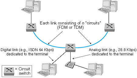Figure 1.5: A simple circuit-switched network consisting of three circuit switches interconnected with two links

Multiplexing

A circuit in a link is implemented with either frequency-division multiplexing (FDM) or time-division multiplexing (TDM). With FDM, the frequency spectrum of a link is shared among the connections established across the link. Specifically, the link dedicates a frequency band to each connection for the duration of the connection. In telephone networks, this frequency band typically has a width of 4 kHz (that is, 4,000 Hertz or 4,000 cycles per second). The width of the band is called, not surprisingly, the bandwidth. FM radio stations also use FDM to share the microwave frequency spectrum.

The trend in modern telephony is to replace FDM with TDM. Most links in most telephone systems in the United States and in other developed countries currently employ TDM. For a TDM link, time is divided into frames of fixed duration, and each frame is divided into a fixed number of time slots. When the network establishes a connection across a link, the network dedicates one time slot in every frame to the connection. These slots are dedicated for the sole use of that connection, with a time slot available for use (in every frame) to transmit the connection's data.

Figure 1.6 illustrates FDM and TDM for a specific network link. For FDM, the frequency domain is segmented into a number of circuits, each of bandwidth 4 kHz. For TDM, the time domain is segmented into four circuits; each circuit is assigned the same dedicated slot in the revolving TDM frames. The transmission rate of each circuit is equal to the frame rate multiplied by the number of bits in a slot. For example, if the link transmits 8,000 frames per second and each slot consists of 8 bits, then the circuit transmission rate is 64Kbps.

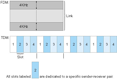Figure 1.6: With FDM, each circuit continuously gets a fraction of the bandwidth. With TDM, each circuit gets all of the bandwidth periodically during brief intervals of time (that is, during slots).

Proponents of packet switching have always argued that circuit switching is wasteful because the dedicated circuits are idle during silent periods. For example, when one of the conversants in a telephone call stops talking, the idle network resources (frequency bands or slots in the links along the connection's route) cannot be used by other ongoing connections. As another example of how these resources can be underutilized, consider a radiologist who uses a circuit-switched network to remotely access a series of x-rays. The radiologist sets up a connection, requests an image, contemplates the image, and then requests a new image. Network resources are wasted during the radiologist's contemplation periods. Proponents of packet switching also enjoy pointing out that establishing end-to-end circuits and reserving end-to-end bandwidth is complicated and requires complex signaling software to coordinate the operation of the switches along the end-to-end path.

Before we finish our discussion of circuit switching, let's work through a numerical example that should shed further insight on the matter. Let us consider how long it takes to send a file of 640 Kbits from host A to host B over a circuit-switched network. Suppose that all links in the network use TDM with 24 slots and have a bit rate of 1.536 Mbps. Also suppose that it takes 500 msec to establish an end-to-end circuit before A can begin to transmit the file. How long does it take to send the file? Each circuit has a transmission rate of (1.536 Mbps)/24 = 64 Kbps, so it takes (640 Kbits)/(64 Kbps) = 10 seconds to transmit the file. To this 10 seconds we add the circuit establishment time, giving 10.5 seconds to send the file. Note that the transmission time is independent of the number of links. The transmission time would be 10 seconds if the end-to-end circuit passes through one link or one hundred links. (The actual end-to-end delay also includes a propagation delay; see Section 1.6). AT&T Labs provides an interactive site [AT&T Bandwidth 1999] to explore transmission delay for various file types and transmission technologies.

Packet Switching

We saw in Sections 1.2 and 1.3 that application-level protocols exchange messages in accomplishing their task. Messages can contain anything the protocol designer desires. Messages may perform a control function (for example, the "Hi" messages in our handshaking example) or can contain data, such as an ASCII file, a Postscript file, a Web page, or a digital audio file. In modern packet-switched networks, the source breaks long messages into smaller packets. Between source and destination, each of these packets traverse communication links and packet switches (also known as routers). Packets are transmitted over each communication link at a rate equal to the full transmission rate of the link. Most packet switches use store-and-forward transmission at the inputs to the links. Store-and-forward transmission means that the switch must receive the entire packet before it can begin to transmit the first bit of the packet onto the outbound link. Thus store-and-forward packet switches introduce a store-and-forward delay at the input to each link along the packet's route. This delay is proportional to the packet's length in bits. In particular, if a packet consists of L bits, and the packet is to be forwarded onto an outbound link of R bps, then the store-and-forward delay at the switch is L/R seconds.

Within each router there are multiple buffers (also called queues), with each link having an input buffer (to store packets that have just arrived to that link) and an output buffer. The output buffers play a key role in packet switching. If an arriving packet needs to be transmitted across a link but finds the link busy with the transmission of another packet, the arriving packet must wait in the output buffer. Thus, in addition to the store-and-forward delays, packets suffer output buffer queuing delays. These delays are variable and depend on the level of congestion in the network. Since the amount of buffer space is finite, an arriving packet may find that the buffer is completely filled with other packets waiting for transmission. In this case, packet loss will occur--either the arriving packet or one of the already-queued packets will be dropped. Returning to our restaurant analogy from earlier in this section, the queuing delay is analogous to the amount of time one spends waiting for a table. Packet loss is analogous to being told by the waiter that you must leave the premises because there are already too many other people waiting at the bar for a table.

Figure 1.7 illustrates a simple packet-switched network. Suppose Hosts A and B are sending packets to Host E. Hosts A and B first send their packets along the 10 Mbps link to the first packet switch. The packet switch directs these packets to the 1.544 Mbps link. If there is congestion at this link, the packets queue in the link's output buffer before they can be transmitted onto the link. Consider now how Host A and Host B packets are transmitted onto this link. As shown in Figure 1.7, the sequence of A and B packets does not follow any periodic ordering; the ordering is random or statistical because packets are sent whenever they happen to be present at the link. For this reason, we often say that packet switching employs statistical multiplexing. Statistical multiplexing sharply contrasts with time-division multiplexing (TDM), for which each host gets the same slot in a revolving TDM frame.

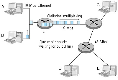Figure 1.7: Packet switching

Let us now consider how long it takes to send a packet of L bits from one host to another host across a packet-switched network. Let us suppose that there are Q links between the two hosts, each of rate R bps. Assume that queuing delays and end-to-end propagation delays are negligible and that there is no connection establishment. The packet must first be transmitted onto the first link emanating from host A; this takes L/R seconds. It must then be transmitted on each of the Q-1 remaining links, that is, it must be stored and forwarded Q-1 times. Thus the total delay is QL/R.

Packet Switching versus Circuit Switching

Having described circuit switching and packet switching, let us compare the two. Opponents of packet switching have often argued that packet switching is not suitable for real-time services (for example, telephone calls and video conference calls) because of its variable and unpredictable delays. Proponents of packet switching argue that (1) it offers better sharing of bandwidth than circuit switching and (2) it is simpler, more efficient, and less costly to implement than circuit switching. Generally speaking, people who do not like to hassle with restaurant reservations prefer packet switching to circuit switching.

Why is packet switching more efficient? Let us look at a simple example. Suppose users share a 1 Mbps link. Also suppose that each user alternates between periods of activity (when it generates data at a constant rate of 100 Kbps) and periods of inactivity (when it generates no data). Suppose further that a user is active only 10 percent of the time (and is idle drinking coffee during the remaining 90 percent of the time). With circuit switching, 100 Kbps must be reserved for each user at all times. Thus, the link can support only 10 simultaneous users. With packet switching, if there are 35 users, the probability that there are more than 10 simultaneously active users is approximately 0.0004. If there are 10 or fewer simultaneously active users (which happens with probability 0.9996), the aggregate arrival rate of data is less than or equal to 1 Mbps (the output rate of the link). Thus, users' packets flow through the link essentially without delay, as is the case with circuit switching. When there are more than 10 simultaneously active users, then the aggregate arrival rate of packets will exceed the output capacity of the link, and the output queue will begin to grow (until the aggregate input rate falls back below 1 Mbps, at which point the queue will begin to diminish in length). Because the probability of having 10 or more simultaneously active users is very very small, packet-switching almost always has the same delay performance as circuit switching, but does so while allowing for more than three times the number of users.

Although packet switching and circuit switching are both very prevalent in today's telecommunication networks, the trend is certainly in the direction of packet switching. Even many of today's circuit-switched telephone networks are slowly migrating towards packet switching. In particular, telephone networks often convert to packet switching for the expensive overseas portion of a telephone call.

Message Switching

In a modern packet-switched network, the source host segments long messages into smaller packets and sends the smaller packets into the network; the receiver reassembles the packets back into the original message. But why bother to segment the messages into packets in the first place, only to have to reassemble packets into messages? Doesn't this place an additional and unnecessary burden on the source and destination? Although the segmentation and reassembly do complicate the design of the source and receiver, researchers and network designers concluded in the early days of packet switching that the advantages of segmentation greatly compensate for its complexity. Before discussing some of these advantages, we need to introduce some terminology. We say that a packet-switched network performs message switching if the sources do not segment messages (that is, they send a message into the network as a whole). Thus message switching is a specific kind of packet switching, whereby the packets traversing the network are themselves entire messages.

Figure 1.8 illustrates message switching in a route consisting of two packet switches (PSs) and three links. With message switching, the message stays intact as it traverses the network. Because the switches are store-and-forward packet switches, a packet switch must receive the entire message before it can begin to forward the message on an outbound link.

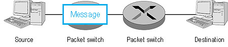Figure 1.8: A simple message-switched network

Figure 1.9 illustrates packet switching for the same network. In this example, the original message has been divided into five distinct packets. In Figure 1.9, the first packet has arrived at the destination, the second and third packets are in transit in the network, and the last two packets are still in the source. Again, because the switches are store-and-forward packet switches, a packet switch must receive an entire packet before it can begin to forward the packet on an outbound link.

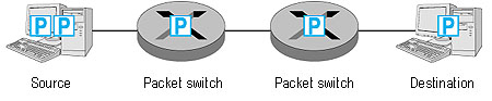Figure 1.9: A simple packet-switched network

One major advantage of packet switching (with segmented messages) is that it achieves end-to-end delays that are typically much smaller than the delays associated with message switching. We illustrate this point with the following simple example. Consider a message that is 7.5 Mbits long. Suppose that between source and destination there are two packet switches and three links, and that each link has a transmission rate of 1.5 Mbps. Assuming there is no congestion in the network, how much time is required to move the message from source to destination with message switching? It takes the source 5 seconds to move the message from the source to the first switch. Because the switches use store-and-forward transmission, the first switch cannot begin to transmit any bits in the message onto the link until this first switch has received the entire message. Once the first switch has received the entire message, it takes 5 seconds to move the message from the first switch to the second switch. Thus it takes 10 seconds to move the message from the source to the second switch. Following this logic we see that a total of 15 seconds is needed to move the message from source to destination. These delays are illustrated in Figure 1.10.

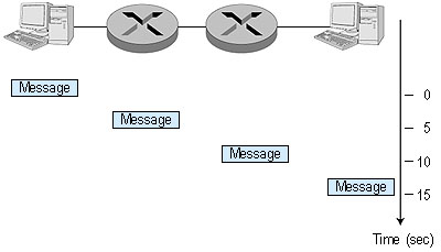Figure 1.10: Timing of message transfer of a 7.5 Mbit message in a message-switched network

Continuing with the same example, now suppose that the source breaks the message into 5,000 packets, with each packet being 1.5 Kbits long. Again assuming that there is no congestion in the network, how long does it take to move the 5,000 packets from source to destination? It takes the source 1 msec to move the first packet from the source to the first switch. And it takes the first switch 1 msec to move this first packet from the first to the second switch. But while the first packet is being moved from the first switch to the second switch, the second packet is simultaneously moved from the source to the first switch. Thus the second packet reaches the first switch at time = 2 msec. Following this logic we see that the last packet is completely received at the first switch at time = 5,000 msec = 5 seconds. Since this last packet has to be transmitted on two more links, the last packet is received by the destination at 5.002 seconds (see Figure 1.11).

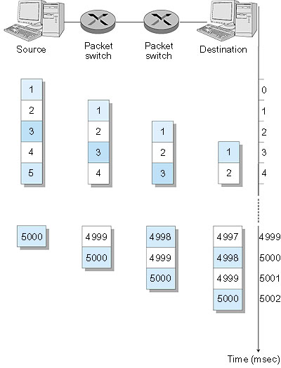Figure 1.11: Timing of packet transfer of a 7.5 Mbit message, divided into 5,000 packets, in a packet-switched network

Amazingly enough, packet switching has reduced the message-switching delay by a factor of three! But why is this so? What is packet switching doing that is different from message switching? The key difference is that message switching is performing sequential transmission whereas packet switching is performing parallel transmission. Observe that with message switching, while one node (the source or one of the switches) is transmitting, the remaining nodes are idle. With packet switching, once the first packet reaches the last switch, three nodes transmit at the same time.

Packet switching has yet another important advantage over message switching. As we will discuss later in this book, bit errors can be introduced into packets as they transit the network. When a switch detects an error in a packet, it typically discards the entire packet. So, if the entire message is a packet and one bit in the message gets corrupted, the entire message is discarded. If, on the other hand, the message is segmented into many packets and one bit in one of the packets is corrupted, then only that one packet is discarded.

Packet switching is not without its disadvantages, however. We will see that each packet or message must carry, in addition to the data being sent from the sending application to the receiving application, an amount of control information. This information, which is carried in the packet or message header, might include the identity of the sender and receiver and a packet or message identifier (for example, number). Since the amount of header information would be approximately the same for a message or a packet, the amount of header overhead per byte of data is higher for packet switching than for message switching.

Before moving on to the next subsection, you are highly encouraged to explore the Message-Switching Java Applet. Click here to open it in a new window, or select it from the menu bar at the left. This applet will allow you to experiment with different message and packet sizes, and will allow you to examine the effect of additional propagation delays.

1.4.2: Routing in Data Networks

There are two broad classes of packet-switched networks: datagram networks and virtual circuit networks. They differ according to whether they route packets according to host destination addresses or according to virtual circuit numbers. We shall call any network that routes packets according to host destination addresses a datagram network. The IP protocol of the Internet routes packets according to the destination addresses; hence the Internet is a datagram network. We shall call any network that routes packets according to virtual circuit numbers a virtual circuit network. Examples of packet-switching technologies that use virtual circuits include X.25, frame relay, and ATM (asynchronous transfer mode).

Virtual Circuit Networks

A virtual circuit (VC) consists of (1) a path (that is, a series of links and packet switches) between the source and destination hosts, (2) virtual circuit numbers, one number for each link along the path, and (3) entries in VC-number translation tables in each packet switch along the path. Once a VC is established between source and destination, packets can be sent with the appropriate VC numbers. Because a VC has a different VC number on each link, an intermediate packet switch must replace the VC number of each traversing packet with a new one. The new VC number is obtained from the VC-number translation table.

To illustrate the concept, consider the network shown in Figure 1.12. Suppose host A requests that the network establish a VC between itself and host B. Suppose that the network chooses the path A-PS1-PS2-B and assigns VC numbers 12, 22, 32 to the three links in this path. Then, when a packet as part of this VC leaves host A, the value in the VC-number field is 12; when it leaves PS1, the value is 22; and when it leaves PS2, the value is 32. The numbers next to the links of PS1 are the interface numbers.

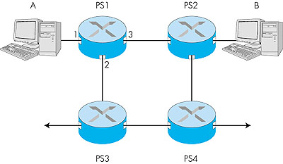Figure 1.12: A simple virtual circuit network

How does the switch determine the replacement VC number for a packet traversing the switch? Each switch has a VC-number translation table; for example, the VC-number translation table in PS1 might look something like this:

Whenever a new VC is established across a switch, an entry is added to the VC-number table. Similarly, whenever a VC terminates, the entries in each table along its path are removed.

You might be wondering why a packet doesn't just keep the same VC number on each of the links along its route. The answer is twofold. First, by replacing the number from link to link, the length of the VC field is reduced. Second, and more importantly, by permitting a different VC number for each link along the path of the VC, a network management function is simplified. Specifically, with multiple VC numbers, each link in the path can choose a VC number independently of what the other links in the path chose. If a common number were required for all links along the path, the switches would have to exchange and process a substantial number of messages to agree on the VC number to be used for a connection.

If a network employs virtual circuits, then the network's switches must maintain state information for the ongoing connections. Specifically, each time a new connection is established across a switch, a new connection entry must be added to the switch's VC-number translation table; and each time a connection is released, an entry must be removed from the table. Note that even if there is no VC-number translation, it is still necessary to maintain state information that associates VC numbers to interface numbers. The issue of whether or not a switch or router maintains state information for each ongoing connection is a crucial one--one that we return to shortly below.

Datagram Networks

Datagram networks are analogous in many respects to the postal services. When a sender sends a letter to a destination, the sender wraps the letter in an envelope and writes the destination address on the envelope. This destination address has a hierarchical structure. For example, letters sent to a location in the United States include the country (USA), the state (for example, Pennsylvania), the city (for example, Philadelphia), the street (for example, Walnut Street) and the number of the house on the street (for example, 421). The postal services use the address on the envelope to route the letter to its destination. For example, if the letter is sent from France, then a postal office in France will first direct the letter to a postal center in the United States. This postal center in the United States will then send the letter to a postal center in Philadelphia. Finally, a mail person working in Philadelphia will deliver the letter to its ultimate destination.

In a datagram network, each packet that traverses the network contains in its header the address of the destination. As with postal addresses, this address has a hierarchical structure. When a packet arrives at a packet switch in the network, the packet switch examines a portion of the packet's destination address and forwards the packet to an adjacent switch. More specifically, each packet switch has a routing table that maps destination addresses (or portions of the destination addresses) to an outbound link. When a packet arrives at a switch, the switch examines the address and indexes its table with this address to find the appropriate outbound link. The switch then sends the packet into this outbound link.

The whole routing process is also analogous to the car driver who does not use maps but instead prefers to ask for directions. For example, suppose Joe is driving from Philadelphia to 156 Lakeside Drive in Orlando, Florida. Joe first drives to his neighborhood gas station and asks how to get to 156 Lakeside Drive in Orlando, Florida. The gas station attendant extracts the Florida portion of the address and tells Joe that he needs to get onto the interstate highway I-95 South, which has an entrance just next to the gas station. He also tells Joe that once he enters Florida he should ask someone else there. Joe then takes I-95 South until he gets to Jacksonville, Florida, at which point he asks another gas station attendant for directions. The attendant extracts the Orlando portion of the address and tells Joe that he should continue on I-95 to Daytona Beach and then ask someone else. In Daytona Beach another gas station attendant also extracts the Orlando portion of the address and tells Joe that he should take I-4 directly to Orlando. Joe takes I-4 and gets off at the Orlando exit. Joe goes to another gas station attendant, and this time the attendant extracts the Lakeside Drive portion of the address and tells Joe the road he must follow to get to Lakeside Drive. Once Joe reaches Lakeside Drive he asks a kid on a bicycle how to get to his destination. The kid extracts the 156 portion of the address and points to the house. Joe finally reaches his ultimate destination.

We will be discussing routing in datagram networks in great detail in this book. But for now we mention that, in contrast with VC networks, datagram networks do not maintain connection-state information in their switches. In fact, a switch in a pure datagram network is completely oblivious to any flows of traffic that may be passing through it--it makes routing decisions for each individual packet. Because VC networks must maintain connection-state information in their switches, opponents of VC networks argue that VC networks are overly complex. These opponents include most researchers and engineers in the Internet community. Proponents of VC networks feel that VCs can offer applications a wider variety of networking services.

How would you like to actually see the route that packets take in the Internet? We now invite you to get your hands dirty by interacting with the Traceroute program, using the interface provided. Click here to open it in a new window, or select it from the menu bar at the left.

Network Taxonomy

We have now introduced several important networking concepts: circuit switching, packet switching, message switching, virtual circuits, connectionless service, and connection-oriented service. How does it all fit together?

First, in our simple view of the world, a telecommunications network either employs circuit switching or packet switching (see Figure 1.13). A link in a circuit-switched network can employ either FDM or TDM (see Figure 1.14). Packet-switched networks are either virtual circuit networks or datagram networks. Switches in virtual circuit networks route packets according to the packets' VC numbers and maintain connection state. Switches in datagram networks route packets according to the packets' destination addresses and do not maintain connection state (see Figure 1.15).

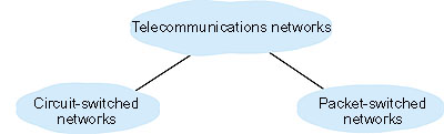Figure 1.13: Highest-level distinction among telecommunication networks: Circuit-switched or packet-switched?

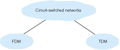Figure 1.14: Circuit-switching implementations: FDM or TDM?

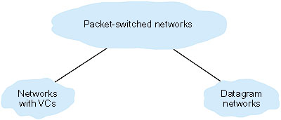Figure 1.15: Packet-switching implementation: Virtual circuits or datagrams?

Examples of packet-switched networks that use VCs include X.25, frame relay, and ATM. A packet-switched network either (1) uses VCs for all of its message routing, or (2) uses destination addresses for all of its message routing. It doesn't employ both routing techniques. (This last statement is a bit of a white lie, as there are networks that use datagram routing "on top of" VC routing. This is the case for "IP over ATM," as we shall cover later in the book.)

A datagram network is not, however, either a connectionless or a connection-oriented network. Indeed, a datagram network can provide the connectionless service to some of its applications and the connection-oriented service to other applications. For example, the Internet, which is a datagram network, provides both connectionless and connection-oriented service to its applications. We saw in Section 1.3 that these services are provided in the Internet by the UDP and TCP protocols, respectively. Networks with VCs--such as X.25, Frame Relay, and ATM--are always, however, connection-oriented.